Science and engineering increasingly simulate systems that cross domains, and each domain brings its own mathematics: linear algebra for structures, conservation laws for flow, Clifford algebra for spinors. In code, each often arrives as a separate library with its own conventions: row-major or column-major storage, zero-based or one-based indices, one sign convention for the spacetime metric or the other, and a number type its author fixed in advance. A crossing between two libraries with different conventions needs translation code, and each translation is a place where an error can pass unnoticed.
Unified math replaces the translation with composition. Seventeen open-source crates in DeepCausality form one stack: a hierarchy of algebraic traits states the laws a number obeys, and an interface from category theory states how containers compose. A tensor of multivectors is then an ordinary type, and a single call rotates every cell of a vector field by a Clifford rotor.
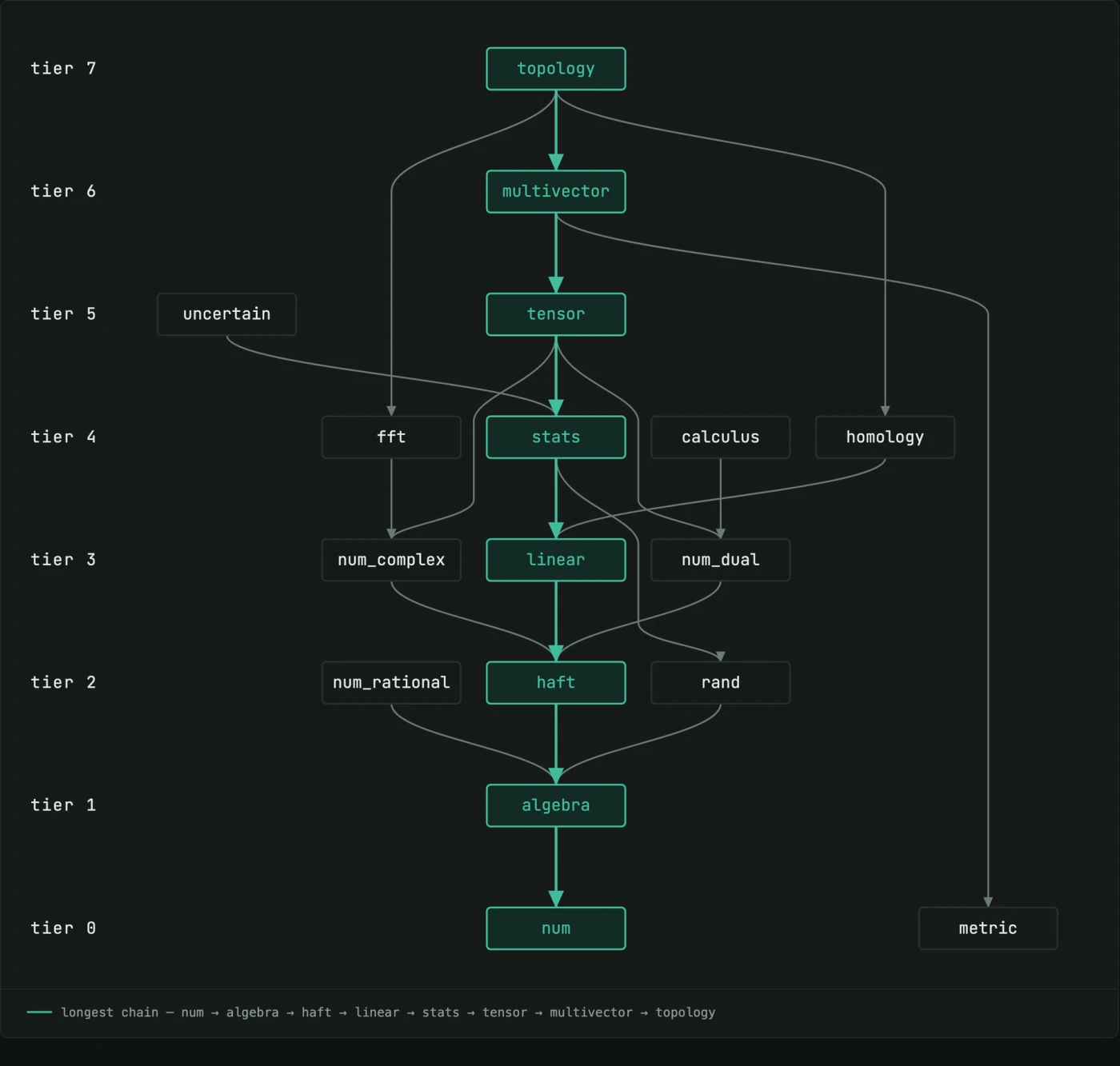
Laws in the types
A type declares the algebraic laws it satisfies, and an algorithm declares the laws it needs. The compiler rejects a mismatch, so a routine that requires associativity accepts only types that declare it. Floating-point types declare the laws of the real numbers they approximate. The traits cover the natural numbers through the octonions, and each number system stops where its mathematics does: the integers form a Euclidean domain, not a field. One crate defines the metric signatures, and every multivector carries one: the general constructor takes it as an argument, and named constructors, such as the one for spacetime algebra, fix it. Lean proofs check the monad and Kleisli laws behind the composition.
Precision as a parameter
Every crate above the base is generic in its scalar, so a program names its working type in one line. Change that line, and every computation written against it runs at one of four precisions. The last column sums a million terms of a series whose value is known and counts the digits each type gets right.
| Type | Size | Significand | Machine ε | Decimal digits | Largest finite | Correct digits in the test sum |
|---|---|---|---|---|---|---|
| BFloat16 | 2 bytes | 8 bits | 7.8 × 10⁻³ | 2 | 3.4 × 1038 | 2 |
| f32 | 4 bytes | 24 bits | 1.2 × 10⁻⁷ | 7 | 3.4 × 1038 | 4 |
| f64 | 8 bytes | 53 bits | 2.2 × 10⁻¹⁶ | 16 | 1.8 × 10308 | 13 |
| Float106 | 16 bytes | 106 bits | 4.9 × 10⁻³² | 31 | 1.8 × 10308 | 30 |
Parts of one program can also run at different precisions. A Monte Carlo estimate limited by statistical noise gains nothing from extra bits, so it runs in f32 and stores its draws in a quarter of the memory Float106 would need. A reference sum runs in Float106. The two results meet at the wider precision without loss.
Why two of the types are built in software
Float106 exists for precision. It stores each value as the unevaluated sum of two f64 values. That gives it twice the significand of f64 but the same exponent, and so the same range. It runs on ordinary f64 hardware at roughly two to four times the cost of f64. IEEE quadruple precision, f128, offers more: a 113-bit significand, a range to about 104932, and correctly rounded operations. Outside IBM's POWER9 and later processors, though, f128 runs emulated in software, usually slower than Float106. For a calculation that stays within the range of f64 and needs more digits, Float106 is the cheaper choice today.
BFloat16 exists to save memory in AI models. It halves the memory of f32 for weights and activations and keeps f32's eight exponent bits, so it holds the same magnitudes with fewer digits. Its buffers are byte-compatible with the bf16 data that accelerators exchange. IEEE half precision, f16, splits the same two bytes differently. Its 11-bit significand gives about three decimal digits instead of two, but its 5-bit exponent caps the range at 65,504, so values outside that band overflow or vanish unless the program rescales them.
Rust's own f16 and f128 types are still in development. Once they become available, unified math needs a minor patch in one place, the numeric base crate, to support both; every crate above it takes the new float types as a parameter.
The value of unified math
Unified math pays off in two ways. A coupled model built on the stack needs no translation code between its parts, so it has one fewer place to go wrong. And because precision is a parameter, a modeler can measure rounding error instead of assuming it: rerun a deterministic model at a second precision, and the parts whose results move are the parts that rounding limits. A single computation shows both benefits.
The computation is a common one: an integral together with its derivative with respect to a parameter, such as the derivative of ∫01 sin(θx) dx with respect to θ. Conventional code gets that derivative in one of three ways: by hand, by integrating twice with a finite-difference step that needs tuning, or through an automatic-differentiation framework.
In the stack, the integrator and the dual numbers compose instead. The quadrature routine is written once, generic in its scalar, and a dual number carries a value together with its derivative. Integrating over dual numbers therefore returns both from a single sweep. This is differentiation under the integral sign, known since Leibniz; here it follows from composing two existing parts, with no code written for the purpose:
pub type FloatType = f64;
const THETA: FloatType = const_scalar_from_float!(FloatType, 1.3);
// ZERO, ONE and PANELS omitted for brevity.

let seeded = Dual::variable(THETA);
let sweep = quadrature(
    |x: Dual<FloatType>| (seeded * x).sin(),
    Dual::constant(ZERO),
    Dual::constant(ONE),
    PANELS,
);
let integral = sweep.value();
let sensitivity = sweep.derivative();
The first line sets the working type for the whole computation. At θ = 1.3 and 128 panels, the sweep returns I(θ) = 0.5634624396 and dI/dθ = 0.3077659585, both matching their closed forms to nine digits.
Changing that first line to Float106 reruns the same sweep at 106 bits. The table lists the error of both results against their closed forms as the number of panels grows. At 128 panels, f64 and Float106 agree, because Simpson's rule, not rounding, limits the result. With more panels, the f64 error falls until it reaches its rounding floor near 10−15 at 8,192 panels; beyond that, each added panel adds rounding error, and the result gets worse. Float106 keeps improving, to about 10−25 at 524,288 panels.
| Panels | Error in the integral I(θ) | Error in the derivative dI/dθ | ||
|---|---|---|---|---|
| f64 | Float106 | f64 | Float106 | |
| 128 | 3.3 × 10⁻¹¹ | 3.3 × 10⁻¹¹ | 1.2 × 10⁻¹⁰ | 1.2 × 10⁻¹⁰ |
| 1,024 | 8.3 × 10⁻¹⁵ | 8.1 × 10⁻¹⁵ | 3.0 × 10⁻¹⁴ | 3.0 × 10⁻¹⁴ |
| 8,192 | 8.9 × 10⁻¹⁶ | 2.0 × 10⁻¹⁸ | 1.7 × 10⁻¹⁶ | 7.2 × 10⁻¹⁸ |
| 65,536 | 4.2 × 10⁻¹⁵ | 4.9 × 10⁻²² | 5.0 × 10⁻¹⁶ | 1.8 × 10⁻²¹ |
| 524,288 | 1.1 × 10⁻¹⁴ | 1.2 × 10⁻²⁵ | 6.8 × 10⁻¹⁵ | 4.3 × 10⁻²⁵ |
Rounding becomes the limit in three common situations. The first is code verification. Engineers check a solver by refining its mesh and confirming that the error falls at the rate the method predicts; in f64, that curve flattens near 10−15 and then turns up, as the table shows. Float106 extends the curve, and its results serve as reference values for testing f64 codes. The second is long integration. Each panel is a step, and orbit propagation, long-duration navigation, and chaotic flow take millions of steps, each adding its rounding error. The third is the small difference of large quantities, such as a clock-rate comparison at the 10−18 level, below the machine epsilon of f64.
The example shows both benefits. The integral and its derivative come from parts that compose without translation, and one changed line separates the error of the method from the error of the arithmetic. The same pattern gives the sensitivity of any integrated quantity, such as accumulated navigation drift or the impulse a burn delivers, to the parameters that shape it.
Open questions
How far composition can reach depends on the laws in the types. A new kind of number enters every algorithm whose requirements its declared laws meet, and no other. Two branches of mathematics that the stack does not yet contain show what that means.
The first, max-plus algebra, replaces addition with the maximum and multiplication with addition. It models systems driven by timing and synchronization, such as scheduled task chains, where matrix products find the longest path through the system: the critical path that sets when it completes. Max-plus numbers have no subtraction, which makes them a semiring rather than a ring. Matrix multiplication in the stack asks only for a commutative semiring, so it would accept them unchanged; row reduction subtracts and divides, so it asks for a field and would reject them. Many algorithms are known to work over a semiring, from shortest-path closures to max-plus eigenvalues; the open work is to bring them into the stack and to find which existing algorithms ask for more laws than they need.
The second, interval arithmetic, computes with ranges guaranteed to contain the exact value. Sampling a navigation or guidance model estimates its outcomes; one run in intervals would bound them all, rounding included. Safety-critical engineering often asks that question: not what usually happens, but what can happen. Intervals would enter the stack as a scalar, like Float106 and the dual numbers, but they obey the distributive law only in part: x(y + z) is contained in xy + xz, and in general not equal to it. Without the distributive law, intervals fall outside the current requirements of matrix multiplication. Admitting intervals means adding a weaker law to the hierarchy or relaxing the requirements of algorithms that stay correct without full distributivity. Tightness is a known difficulty. Interval arithmetic treats every occurrence of a variable as an independent value: for x in [0, 1], it returns [−1, 1] for x − x instead of 0. Over a long computation these overestimates compound, and the bounds widen. Affine arithmetic and Taylor models record how each result depends on the inputs, so x − x comes out as 0 and the bounds usually stay narrower; whether they compose with the stack as cleanly as a plain scalar does is open.
Relation to the other research areas
Dynamic causality builds its causal monad on the same categorical interface; the causal monad lets a simulation pause, fork, and keep an audit log. Counterfactual CFD uses the crates directly and through the DeepCausality physics crate. The quantum causal models behind the Center's quantum sensing and computing research use them directly.
Resources
- Unified Math documentation: the crate map, the algebraic traits, and a worked example across four layers
- Unified Math README on GitHub: the dependency tiers, the witness inventory, and the measured precision tables
- Mathematics examples: runnable programs that combine several crates
← Previous: dynamic causality · All research areas · Next: counterfactual CFD →